Commitment Strategy

Investment Objective

For any investment to be successful, it must align with the investor’s financial goals. Consequently, we start the strategy discussion with defining the investment objective:

• Conservative investment with low volatility
• Suitable for the Investing Toward a Goal and Investing for Income scenarios
• Optimized for high performance at the 5th percentile
• Broad diversification with exposure to stocks, bonds, commodities, and precious metals
• Intuitive mechanism, augmenting a strategic portfolio with tactical features
• Moderate maintenance requirements with a weekly schedule

In other words, the goal for the Commitment strategy is to create a docile investment, appealing to investors looking to meet critical financial goals, or with a low risk-tolerance. Further, we are looking for simple rules, compatible with investors of various mindsets. And finally, the rebalancing schedule should be relaxed enough to accommodate investors with a busy schedule.

In a nutshell, the objective for the Commitment strategy is to be the Swiss army knife of strategies that you cannot go wrong with, pretty much regardless of where you are coming from.

Strategy Construction

Top-Level Architecture

As a starting point for the Commitment strategy, I chose Tony Robbins’ All-Seasons portfolio. I like the portfolio a lot, because of its even-keeled behavior. In fact, the simple buy-and-hold portfolio already outperforms the 60/40 and the S&P 500 at the 5th percentile.

To transform Robbins’ passive asset allocation into a tactical portfolio, Commitment uses two major building blocks:

• Trend-Following
• Risk- and Money-Management

The primary anomaly of the financial markets is the momentum effect. In a nutshell, assets with good historical performance tend to outperform moving forward. Trend-following is closely related to this effect and refers to the notion that assets with rising prices tend to rise further. Consequently, it is possible to reduce investment losses by exiting assets after a period of negative performance. The trend-following module determines which assets are investible, regardless of their position size.

Another empirically observed market anomaly is the phenomenon of volatility clustering. Asset price changes tend to be followed by changes of similar magnitude. Therefore, we can control investment risks by adjusting position sizes based on historical risk metrics. The risk- and money management module calculates the capital allocation for the assets based on a pre-defined risk budget.

Trend-Following

Most investors are familiar with the saying “the trend is your friend.” Unfortunately, implementing this simple idea is more involved than it may seem at first. For a well-performing trend-following mechanism we need to combine two contradictory objectives. For once, the mechanism should react fast enough to avoid sharp losses when markets crash. At the same time, the mechanism needs to be slow enough to avoid whipsaws and unnecessary churn.

There are three main scenarios to consider:

• Markets decline slowly, as they did during the dot-com crash in 2001
• Markets decline quickly, as they did during the subprime lending crisis in 2008, or during the pandemic in 2020
• Markets go sideways with no direction, as observed in 2015 or 2018

In 2001, markets declined slowly enough that there was no noticeable uptick in market volatility. This creates issues with mechanisms that rely on volatility to confirm market reversals.

In 2008 and 2020, markets declined so fast that any lag introduced by the trend-following resulted in painful losses. The need to react swiftly severely limits the amount of filtering that can be applied, forcing strategies to act on noisy data.

In 2015 or 2018, markets went sideways for prolonged periods. As a result, trend-following mechanisms have difficulties deciding on the proper direction, leading to whipsaw losses.

The Commitment strategy’s trend-following consists of three building blocks:

• Moving-average crossover
• Multi-period price regression
• Emergency brake

The simplest of the three modules is the moving-average crossover. This block runs a slow and a fast moving-average on the asset prices and determines bullish conditions whenever the fast average crosses above its slow counterpart. I tuned this part very conservatively, with timing constants of four and six months.

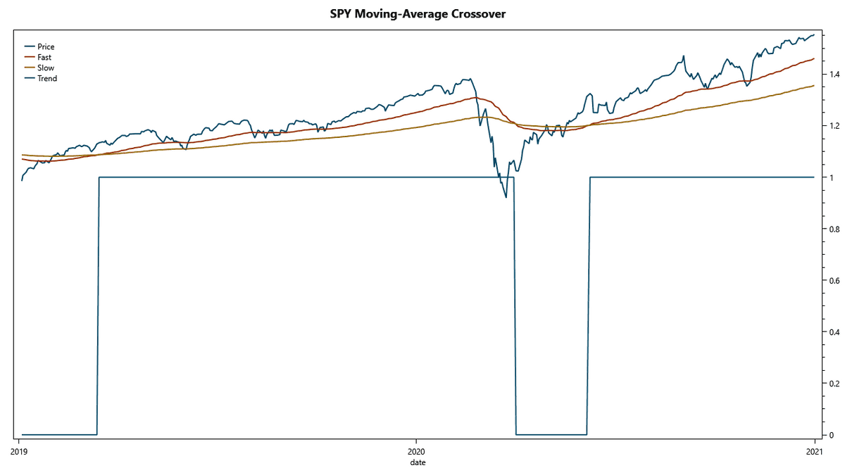
This slow timing prevents the mechanism from whipsaws. However, it is clearly too slow to react to the fast selloffs. The chart above details the 2020 crash. As the pandemic unfolded in 2020, the S&P 500 reached its peak on February 19. On March 23, only 24 trading days later, the index found its bottom about 34% lower.

The moving-average crossover first signaled the market selloff on April 1, when the markets were already recovering from the shock. However, the mechanism has worked sufficiently well to protect investors during the 2001, 2008, and 2020 bear markets. The main value of this mechanism is its simplicity, which makes it an excellent fallback solution.

The second module uses the slope of logarithmic regressions to determine the current trend. By using a swarm of 10 regressions with periods ranging between three and twelve months, the mechanism can self-adjust its timing to the differences between assets and changing market environments.

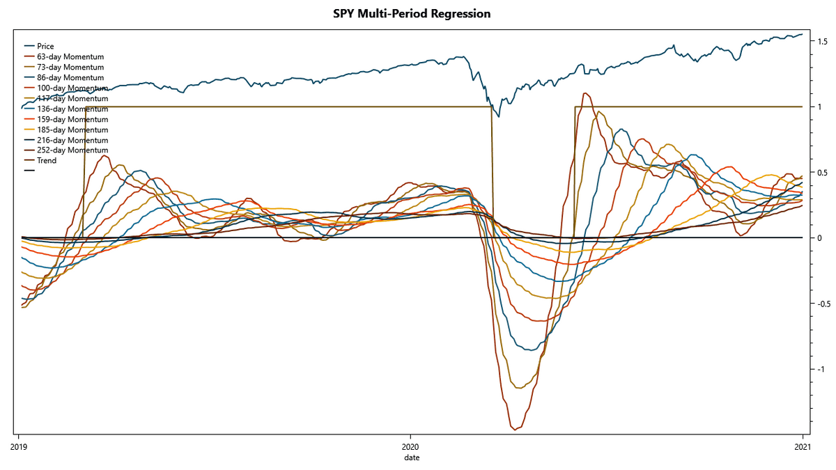
The chart above shows how the swarm of regression slopes, denoting the asset’s momentum over the various timing periods. Some of them are too fast to avoid whipsaws, while others are too slow to prevent deep drawdowns. To consolidate the individual slopes to a single number, the mechanism weighs the various regressions with their R², a value indicating the quality of the regression fit.

This method detected the 2020 crash by March 17, which is two weeks earlier than the moving-average crossover, but still too late to prevent most of the losses. However, this mechanism determined bullish sentiment by June 3, which beats the moving-average crossover by about two weeks. I see the main value of including this mechanism in its ability to self-adjust, making it mostly independent of any tuned parameters and the risk of overfitting.

The previous two trend-following techniques were tuned to reliably detect trends and avoid whipsaws. As we have seen, this comes with significant lag, making the mechanisms too slow to react to fast-paced market selloffs. To overcome this limitation, Commitment comes with an emergency brake mechanism, that evaluates the statistics of recent drawdowns.

This third mechanism calculates the two-year Z-score of the assets’ one-month Ulcer Index. In simple terms, it measures how unusual recent drawdowns were in the historical context. A market crash is detected when the Z-score exceeds two, an event with a probability of about 2.3%. The rationale behind this mechanism is that swift market meltdowns are rare, and consequently come with Ulcer Index readings far out on the tails.

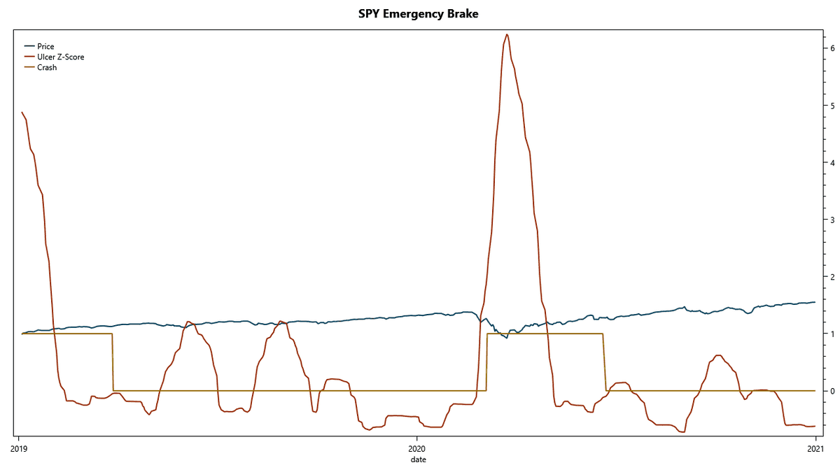
The chart above shows the mechanism’s performance in 2020. The mechanism first detected the market crash on March 6, long before the other two trend-followers. The Z-score peaked at about six, showing that the exact cutoff value is not overly critical. The value of this mechanism is its very fast response, while at the same time being mostly immune to whipsaws.

Trend-Followers	Emergency Brake	Market Exposure
Any state	Crash detected	0%
Both bearish	No crash detected	0%
Mixed bullish/ bearish	No crash detected	50%
Both bullish	No crashdetected	100%

The table above illustrates how I combine the three individual mechanisms into a single signal. The crash-detection overrides the trend-followers, and only allows the strategy to invest in the asset while no crash is detected. Then, the exposure matches the trend-followers’ signals, with the exposure halved in case they disagree.

Risk- and Money-Management

Tony Robbins’ All-Seasons portfolio was inspired by Ray Dalio’s All-Weather strategy. This central idea behind that strategy is to set the weights of the assets such that their risks maintain an intricate balance, a concept called risk-parity. This was implemented in Robbins’ All-Seasons portfolio by setting the asset allocation such that they reflect the assets’ long-term average risks. This is, of course, an oversimplification.

The Commitment strategy adjusts the asset weights dynamically with the goal of controlling the exposure to the various risk factors. This matches the spirit of the All-Weather strategy, even though Bridgewater does not disclose Dalio’s exact algorithm. Calculating the capital allocation is a multi-step process that closely intertwines risk- and money management:

• Determine the strategy’s total risk budget
• Allocate a fraction of risk to each trending asset
• Calculate the capital needs for each asset
• Invest any idle capital in a safe asset

The first step is setting the total risk budget for the strategy. This value is set arbitrarily to 1.5% per day. This seems a lot, as this value exceeds the average risk associated with an investment in the S&P 500. However, on the portfolio level, this will be reduced due to the dampening effects of diversification.

The motivation for keeping the strategy’s risk budget relatively generous is capital utilization. To keep the strategy performing best, it should be constrained by available capital, not risk, under typical circumstances and only start scaling back its position sizes when markets enter turbulent periods.

	Robbins' All-Seasons [% of total capital]	Value at Risk [% of asset value]	ILaP's Commitment [% of total risk budget]
S&P 500	30%	1.3%	40%
30-year Treasury Bonds	40%	0.7%	35%
10-year Treasury Bonds	15%	0.4%	5% (also used as safe-asset)
Gold	7.5%	1.4%	10%
Commodities	7.5%	1.2%	10%
Total	100%		100%

In the next step, Commitment allocates a fraction of the total risk to each asset that is trending up. The baseline risk allocation is derived from Robbins’ All-Seasons portfolio and based on Value at Risk assumptions that match the 30-year average. As this is not an exact science, I rounded the values for convenience.

Of special interest is the case of one or assets trending down. In this case, the remaining assets are scaled up, in an attempt to reach a total of 100%. However, to ensure sufficient diversification, an asset’s risk allocation is limited to no more than twice its baseline allocation or 80% of the total. As a result of these limits, the strategy might not always use the total available risk budget.

Based on the risk allocation, and the asset’s current short-term value at risk, the Commitment strategy now calculates the capital requirements per asset. Oftentimes, when markets are relatively calm, the strategy’s total capital requirements can exceed the available capital. To remedy this situation, the strategy then scales back all positions proportionally.

With rising asset volatility, the position sizes shrink until the available capital is no longer the limiting factor. Instead, the strategy becomes constrained by its risk budget. To avoid idle capital, the strategy assigns any leftover capital to the safe asset. In case it is trending up, this asset is 10-year Treasuries. However, when that asset is bearish, the strategy invests any remaining capital in 3-year Treasury bonds.

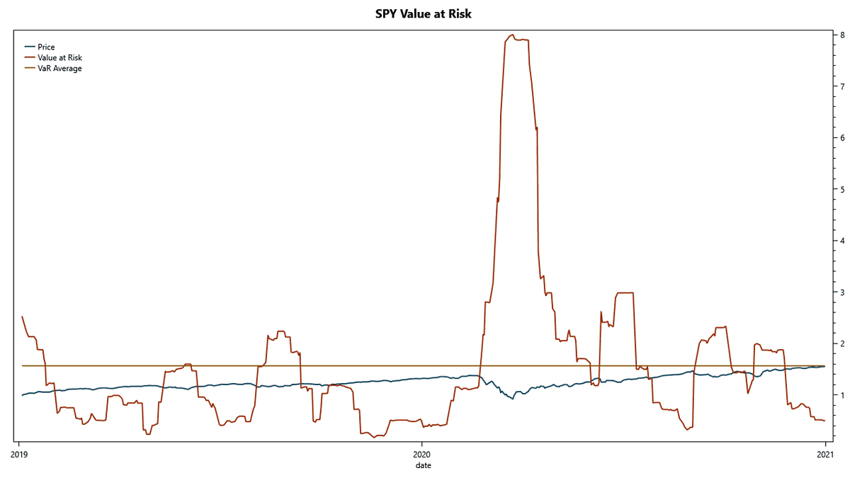
The chart above illustrates the dynamics of value at risk. The long-term average for the stock market is about 1.3%. In 2020, starting February 24, the S&P 500 exceeded the strategy’s overall 1.5% target, leading to a reduction in market exposure. On March 6, the market risk exceeded 3%, leaving less than 50% of the nominal exposure. As a result, this fast-reacting position-sizing can effectively control and reduce the strategy’s risk.

Strategy Results

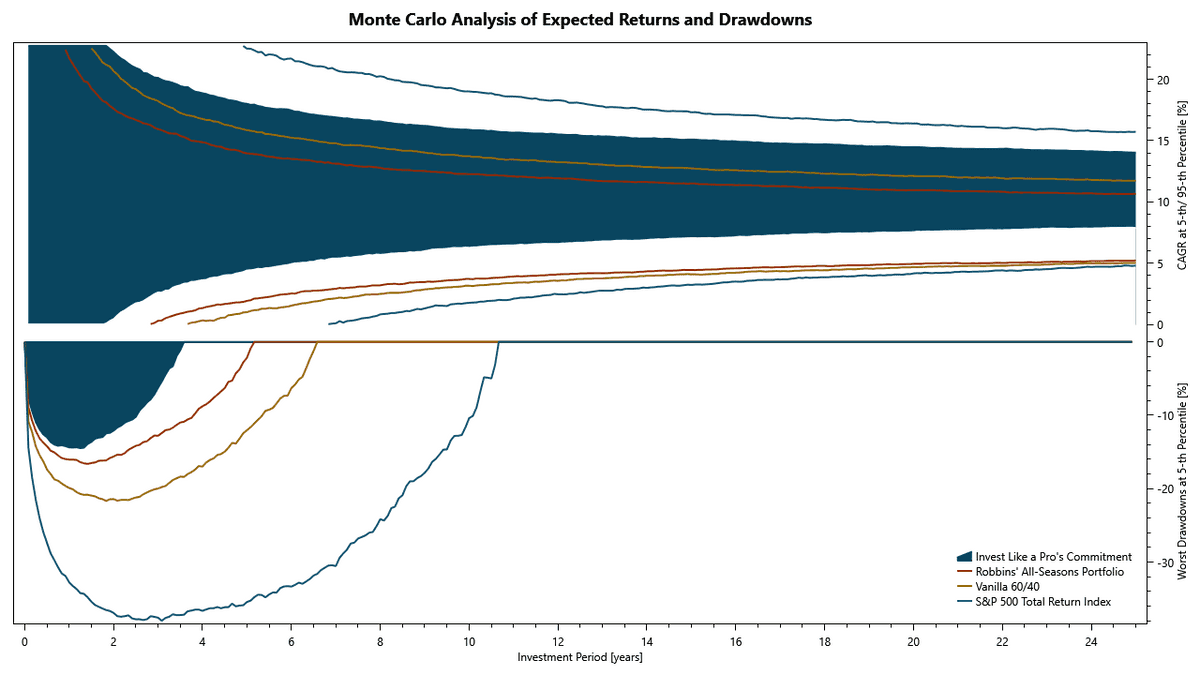
Before looking at the strategy’s results, it is helpful to remind ourselves of the strategy’s main objective: to provide the optimal returns at the 5th percentile. The ex-ante Monte Carlo simulation shows that the _Commitment) strategy delivers on this premise. At the 5th percentile, it beats Robbins’ All-Seasons, the 60/40, and the S&P 500 by a wide margin.

After 25 years, the tactical strategy has a lead of more than 2.5% over its passive cousin, which might not seem much at first. But considering that typical withdrawal rates during retirement are approximately 4%, and that the passive benchmarks come in around 5%, the strategy delivers a substantial edge.

The edge is in no small part owed to the strategy’s money-management, which not only avoids sharp drawdowns, but also keeps capital utilization high. The Monte Carlo simulation shows how the strategy has a 95% probability of breaking even in less than two years: a substantial improvement over the All-Seasons portfolio. Furthermore, the estimated recession drawdowns are not only less deep, but the strategy also recovers from them much faster than the passive benchmark.

While it is comforting for investors to know that their portfolio performs well at the 5th percentile, the Monte Carlo simulation further shows that, in the long term, investors also don’t have to sacrifice any upside when investing in the Commitment strategy. On average, the strategy can rival a buy-and-hold investment in the S&P 500.

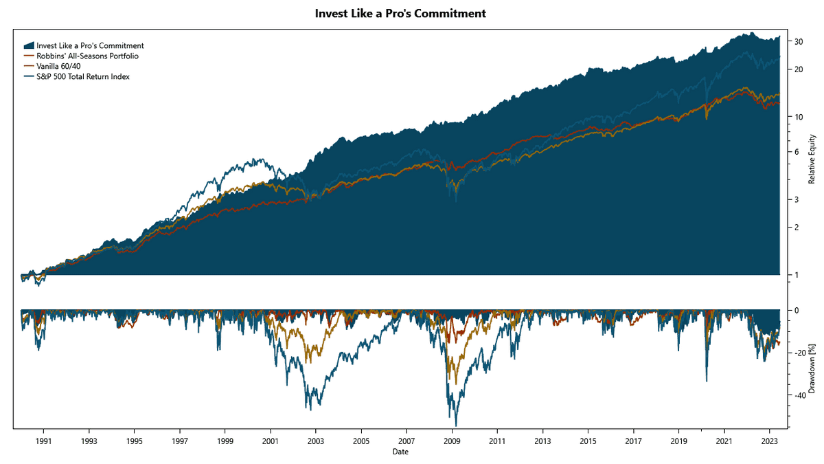
The Monte Carlo simulations paint a somewhat abstract picture of the strategy’s performance. To make the behavior more tangible, it is worth reviewing the backtested equity curve. The simulation shows how the strategy performs admirably well throughout all major drawdowns. Even compared to its passive cousin, the All-Seasons portfolio, the Commitment strategy can further reduce many of the drawdowns. This shows how the combination of trend following and money-management are a valuable improvement upon the strategic portfolio.

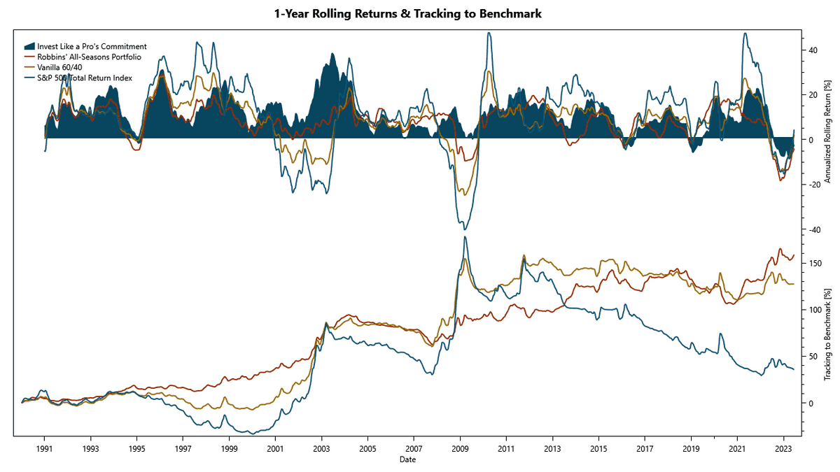
The rolling returns further illustrate the strategy’s ability to avoid or reduce periods of negative returns, except for a few very brief periods. Thanks to this behavior, the strategy can outperform the passive benchmarks in the long term, even though it is often trailing them in the shorter term. In simple words, Commitment is making more by losing less.

The tracking chart further illustrates this. Commitment is steadily leading the All-Seasons, as indicated by the upwards sloping graph. But compared to the 60/40 or the S&P 500, the chart is mostly sloping downwards, indicating Commitment trailing these benchmarks. However, during recession periods, the charts show a sharp step upwards, making up for the previous underperformance.

Metric		Invest Like a Pro's Commitment	Robbins' All-Seasons Portfolio	Vanilla 60/40	S&P 500 Total Return Index
Simulation Start	01/02/1990	$1,000.00	$1,000.00	$1,000.00	$1,000.00
Simulation End	06/14/2023	$32,488.62	$12,278.75	$14,191.01	$24,284.36
Simulation Period	33.4 years
Compound Annual Growth Rate		10.97%	7.79%	8.25%	10.01%
Stdev of Returns (Monthly, Annualized)		8.36%	7.54%	9.28%	14.93%
Maximum Drawdown (Daily)		13.97%	23.62%	35.69%	55.25%
Maximum Flat Days		564.00 days	554.00 days	1281.00 days	2243.00 days
Sharpe Ratio (Rf=T-Bill, Monthly, Annualized)		0.94	0.67	0.59	0.48
Beta (To S&P 500, Monthly)		0.18	0.30	0.61	1.00
Ulcer Index		3.67%	4.30%	7.00%	14.39%
Ulcer Performance Index (Martin Ratio)		2.99	1.81	1.18	0.70

Commitment’s metrics show how the strategy is a substantial improvement, beating its passive benchmarks across the board. Of particular interest are the risk-adjusted returns, measured by the Sharpe Ratio and the Martin Ratio. Further, the low beta indicates how the strategy’s returns are well de-coupled from the stock market as the riskiest ingredient in the asset mix.

Conclusion

In summary, the Commitment strategy is a conservative strategy with low volatility, offering excellent returns at the 5th percentile. With these characteristics, it is an excellent choice for the Investing Toward a Goal and Investing for Income scenarios. Due to its solid average returns, Commitment is also a great fit for risk-averse investors in the Investing Excess Funds scenario.

Most investors should find that the Commitment strategy fits their risk appetite. In the rare case that investors seek to further reduce their investment risk, it can be paired with dedicated low-risk investments, including but not limited to allocating a tranche of their capital to U.S. Treasuries with short maturity.

But performance is not everything. For investors to stay the course even in turbulent times, they also need to agree with the strategy’s methodology. Commitment is an easy choice here. The strategy is based on Tony Robbins’ well-established All-Seasons portfolio, providing instant credibility. Commitment only augments the already great characteristics with an additional tactical layer. The trading rules intuitively make sense and appeal to a wide range of investors, including those skeptical of tactical asset allocation.

To follow the strategy, investors need its weekly asset allocations. While it is possible to code up the strategy by implementing the rules outlined above, such an effort is significantly more involved than investors with a software affinity might initially anticipate. I will discuss this in more detail in the section about implementation. As a reliable solution with a low barrier to entry, TuringTrader.com follows the strategy with daily updated charts and metrics, and, of course, the exact asset allocation.